# (PART) Case studies {-} # Human PBMCs (10X Genomics) ## Introduction This performs an analysis of the public PBMC ID dataset generated by 10X Genomics [@zheng2017massively], starting from the filtered count matrix. ## Data loading ```r library(TENxPBMCData) all.sce <- list( pbmc3k=TENxPBMCData('pbmc3k'), pbmc4k=TENxPBMCData('pbmc4k'), pbmc8k=TENxPBMCData('pbmc8k') ) ``` ## Quality control ```r unfiltered <- all.sce ``` 
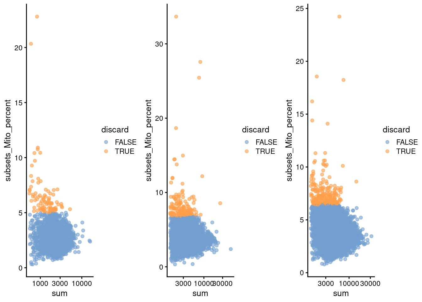
Cell calling implicitly serves as a QC step to remove libraries with low total counts and number of detected genes. Thus, we will only filter on the mitochondrial proportion. ```r library(scater) stats <- high.mito <- list() for (n in names(all.sce)) { current <- all.sce[[n]] is.mito <- grep("MT", rowData(current)$Symbol_TENx) stats[[n]] <- perCellQCMetrics(current, subsets=list(Mito=is.mito)) high.mito[[n]] <- isOutlier(stats[[n]]$subsets_Mito_percent, type="higher") all.sce[[n]] <- current[,!high.mito[[n]]] } ``` ```r qcplots <- list() for (n in names(all.sce)) { current <- unfiltered[[n]] colData(current) <- cbind(colData(current), stats[[n]]) current$discard <- high.mito[[n]] qcplots[[n]] <- plotColData(current, x="sum", y="subsets_Mito_percent", colour_by="discard") + scale_x_log10() } do.call(gridExtra::grid.arrange, c(qcplots, ncol=3)) ```
Percentage of mitochondrial reads in each cell in each of the 10X PBMC datasets, compared to the total count. Each point represents a cell and is colored according to whether that cell was discarded.

(\#fig:unref-pbmc-filtered-var)Percentage of mitochondrial reads in each cell in each of the 10X PBMC datasets, compared to the total count. Each point represents a cell and is colored according to whether that cell was discarded.

```r lapply(high.mito, summary) ``` ``` ## $pbmc3k ## Mode FALSE TRUE ## logical 2609 91 ## ## $pbmc4k ## Mode FALSE TRUE ## logical 4182 158 ## ## $pbmc8k ## Mode FALSE TRUE ## logical 8157 224 ``` ## Normalization We perform library size normalization, simply for convenience when dealing with file-backed matrices. ```r all.sce <- lapply(all.sce, logNormCounts) ``` ```r lapply(all.sce, function(x) summary(sizeFactors(x))) ``` ``` ## $pbmc3k ## Min. 1st Qu. Median Mean 3rd Qu. Max. ## 0.234 0.748 0.926 1.000 1.157 6.604 ## ## $pbmc4k ## Min. 1st Qu. Median Mean 3rd Qu. Max. ## 0.315 0.711 0.890 1.000 1.127 11.027 ## ## $pbmc8k ## Min. 1st Qu. Median Mean 3rd Qu. Max. ## 0.296 0.704 0.877 1.000 1.118 6.794 ``` ## Variance modelling ```r library(scran) all.dec <- lapply(all.sce, modelGeneVar) all.hvgs <- lapply(all.dec, getTopHVGs, prop=0.1) ``` ```r par(mfrow=c(1,3)) for (n in names(all.dec)) { curdec <- all.dec[[n]] plot(curdec$mean, curdec$total, pch=16, cex=0.5, main=n, xlab="Mean of log-expression", ylab="Variance of log-expression") curfit <- metadata(curdec) curve(curfit$trend(x), col='dodgerblue', add=TRUE, lwd=2) } ```
Per-gene variance as a function of the mean for the log-expression values in each PBMC dataset. Each point represents a gene (black) with the mean-variance trend (blue) fitted to the variances.

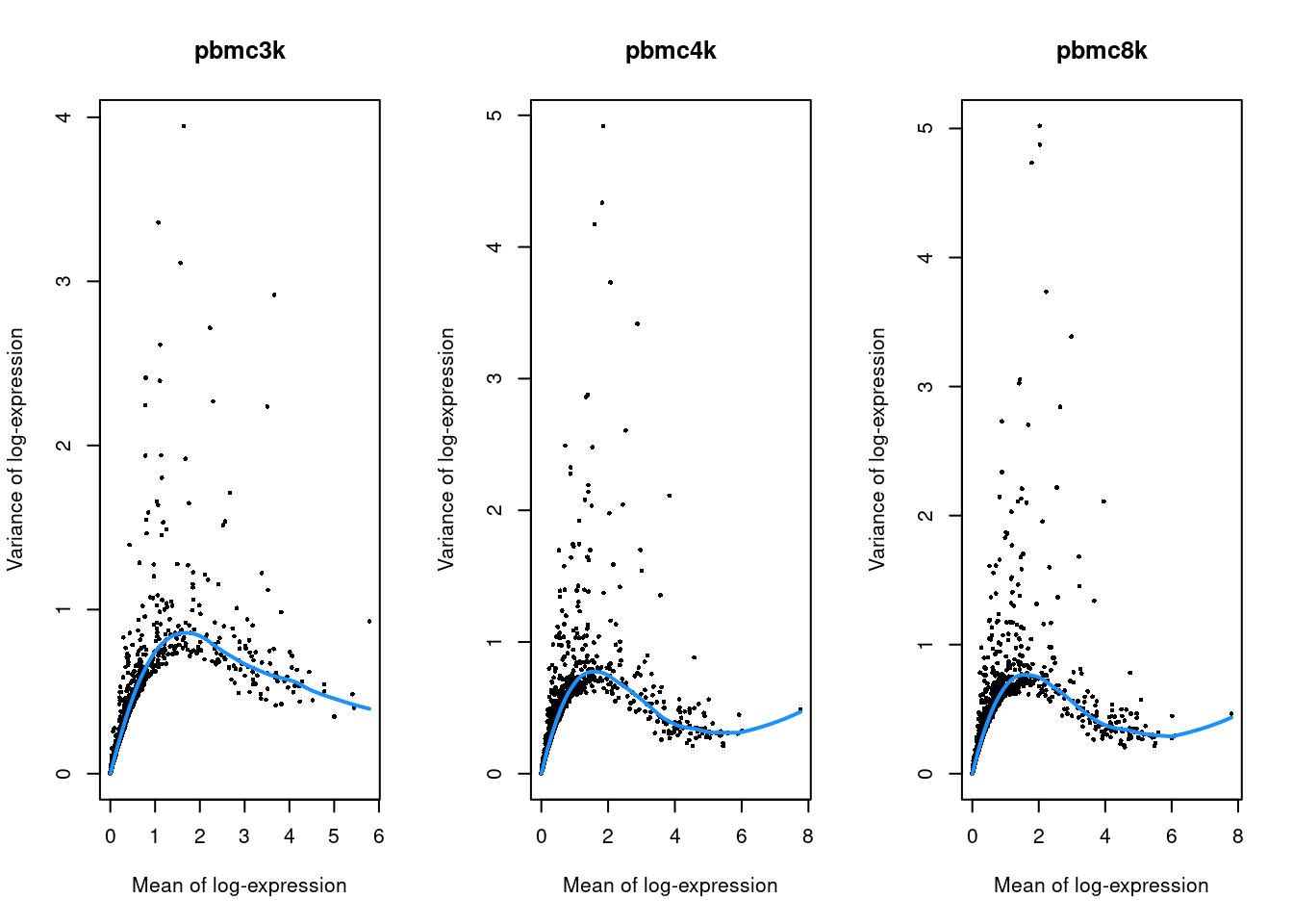
(\#fig:unref-filtered-pbmc-variance)Per-gene variance as a function of the mean for the log-expression values in each PBMC dataset. Each point represents a gene (black) with the mean-variance trend (blue) fitted to the variances.

## Dimensionality reduction For various reasons, we will first analyze each PBMC dataset separately rather than merging them together. We use randomized SVD, which is more efficient for file-backed matrices. ```r library(BiocSingular) set.seed(10000) all.sce <- mapply(FUN=runPCA, x=all.sce, subset_row=all.hvgs, MoreArgs=list(ncomponents=25, BSPARAM=RandomParam()), SIMPLIFY=FALSE) set.seed(100000) all.sce <- lapply(all.sce, runTSNE, dimred="PCA") set.seed(1000000) all.sce <- lapply(all.sce, runUMAP, dimred="PCA") ``` ## Clustering ```r for (n in names(all.sce)) { g <- buildSNNGraph(all.sce[[n]], k=10, use.dimred='PCA') clust <- igraph::cluster_walktrap(g)$membership colLabels(all.sce[[n]]) <- factor(clust) } ``` ```r lapply(all.sce, function(x) table(colLabels(x))) ``` ``` ## $pbmc3k ## ## 1 2 3 4 5 6 7 8 9 10 ## 487 154 603 514 31 150 179 333 147 11 ## ## $pbmc4k ## ## 1 2 3 4 5 6 7 8 9 10 11 12 13 ## 497 185 569 786 373 232 44 1023 77 218 88 54 36 ## ## $pbmc8k ## ## 1 2 3 4 5 6 7 8 9 10 11 12 13 14 15 16 ## 1004 759 1073 1543 367 150 201 2067 59 154 244 67 76 285 20 15 ## 17 18 ## 64 9 ``` ```r all.tsne <- list() for (n in names(all.sce)) { all.tsne[[n]] <- plotTSNE(all.sce[[n]], colour_by="label") + ggtitle(n) } do.call(gridExtra::grid.arrange, c(all.tsne, list(ncol=2))) ```
Obligatory $t$-SNE plots of each PBMC dataset, where each point represents a cell in the corresponding dataset and is colored according to the assigned cluster.

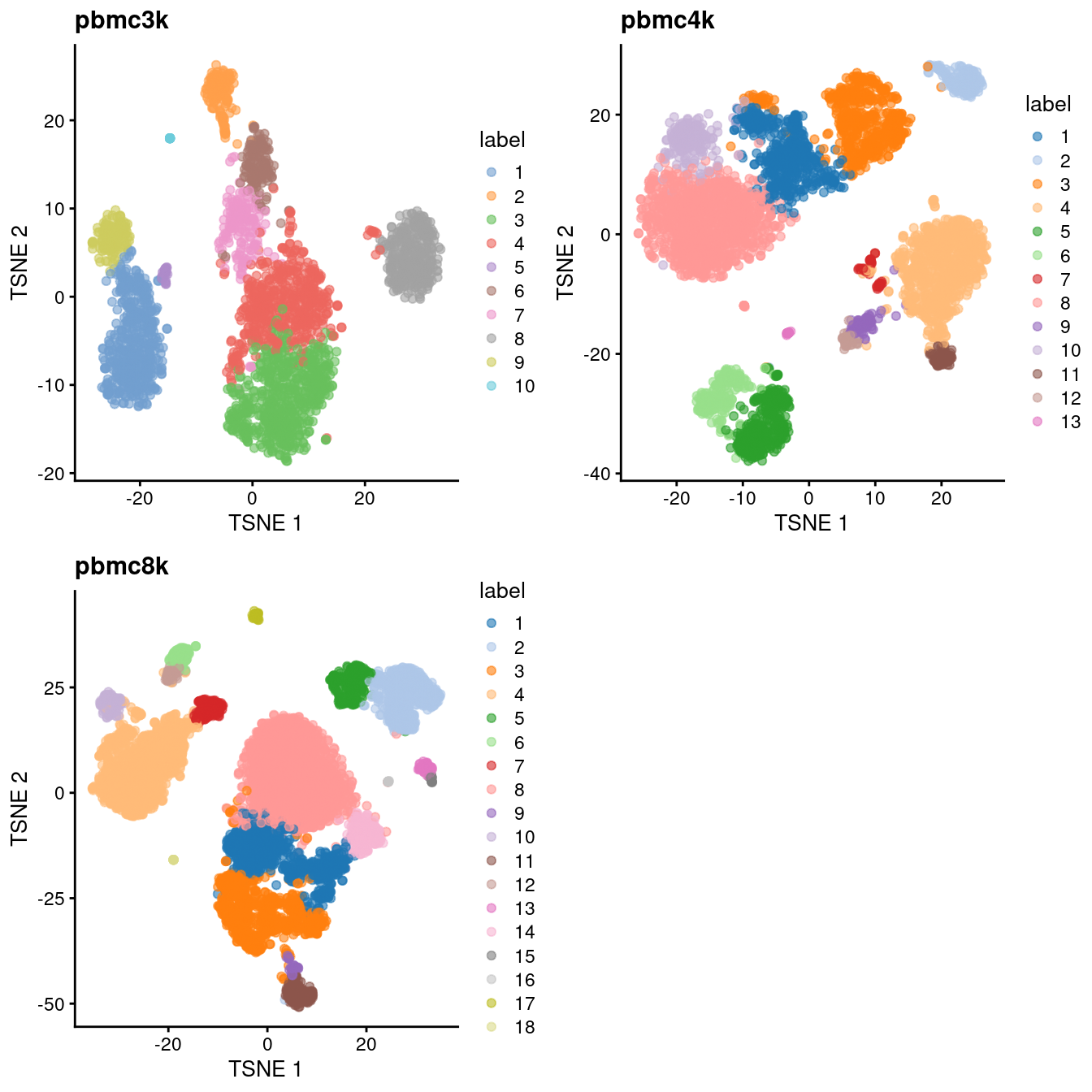
(\#fig:unref-filtered-pbmc-tsne)Obligatory $t$-SNE plots of each PBMC dataset, where each point represents a cell in the corresponding dataset and is colored according to the assigned cluster.

## Data integration With the per-dataset analyses out of the way, we will now repeat the analysis after merging together the three batches. ```r # Intersecting the common genes. universe <- Reduce(intersect, lapply(all.sce, rownames)) all.sce2 <- lapply(all.sce, "[", i=universe,) all.dec2 <- lapply(all.dec, "[", i=universe,) # Renormalizing to adjust for differences in depth. library(batchelor) normed.sce <- do.call(multiBatchNorm, all.sce2) # Identifying a set of HVGs using stats from all batches. combined.dec <- do.call(combineVar, all.dec2) combined.hvg <- getTopHVGs(combined.dec, n=5000) set.seed(1000101) merged.pbmc <- do.call(fastMNN, c(normed.sce, list(subset.row=combined.hvg, BSPARAM=RandomParam()))) ``` We use the percentage of lost variance as a diagnostic measure. ```r metadata(merged.pbmc)$merge.info$lost.var ``` ``` ## pbmc3k pbmc4k pbmc8k ## [1,] 7.003e-03 3.126e-03 0.000000 ## [2,] 7.137e-05 5.125e-05 0.003003 ``` We proceed to clustering: ```r g <- buildSNNGraph(merged.pbmc, use.dimred="corrected") colLabels(merged.pbmc) <- factor(igraph::cluster_louvain(g)$membership) table(colLabels(merged.pbmc), merged.pbmc$batch) ``` ``` ## ## pbmc3k pbmc4k pbmc8k ## 1 113 387 825 ## 2 507 395 806 ## 3 175 344 581 ## 4 295 539 1018 ## 5 346 638 1210 ## 6 11 3 9 ## 7 17 27 111 ## 8 33 113 185 ## 9 423 754 1546 ## 10 4 36 67 ## 11 197 124 221 ## 12 150 180 293 ## 13 327 588 1125 ## 14 11 54 160 ``` And visualization: ```r set.seed(10101010) merged.pbmc <- runTSNE(merged.pbmc, dimred="corrected") gridExtra::grid.arrange( plotTSNE(merged.pbmc, colour_by="label", text_by="label", text_colour="red"), plotTSNE(merged.pbmc, colour_by="batch") ) ```
Obligatory $t$-SNE plots for the merged PBMC datasets, where each point represents a cell and is colored by cluster (top) or batch (bottom).

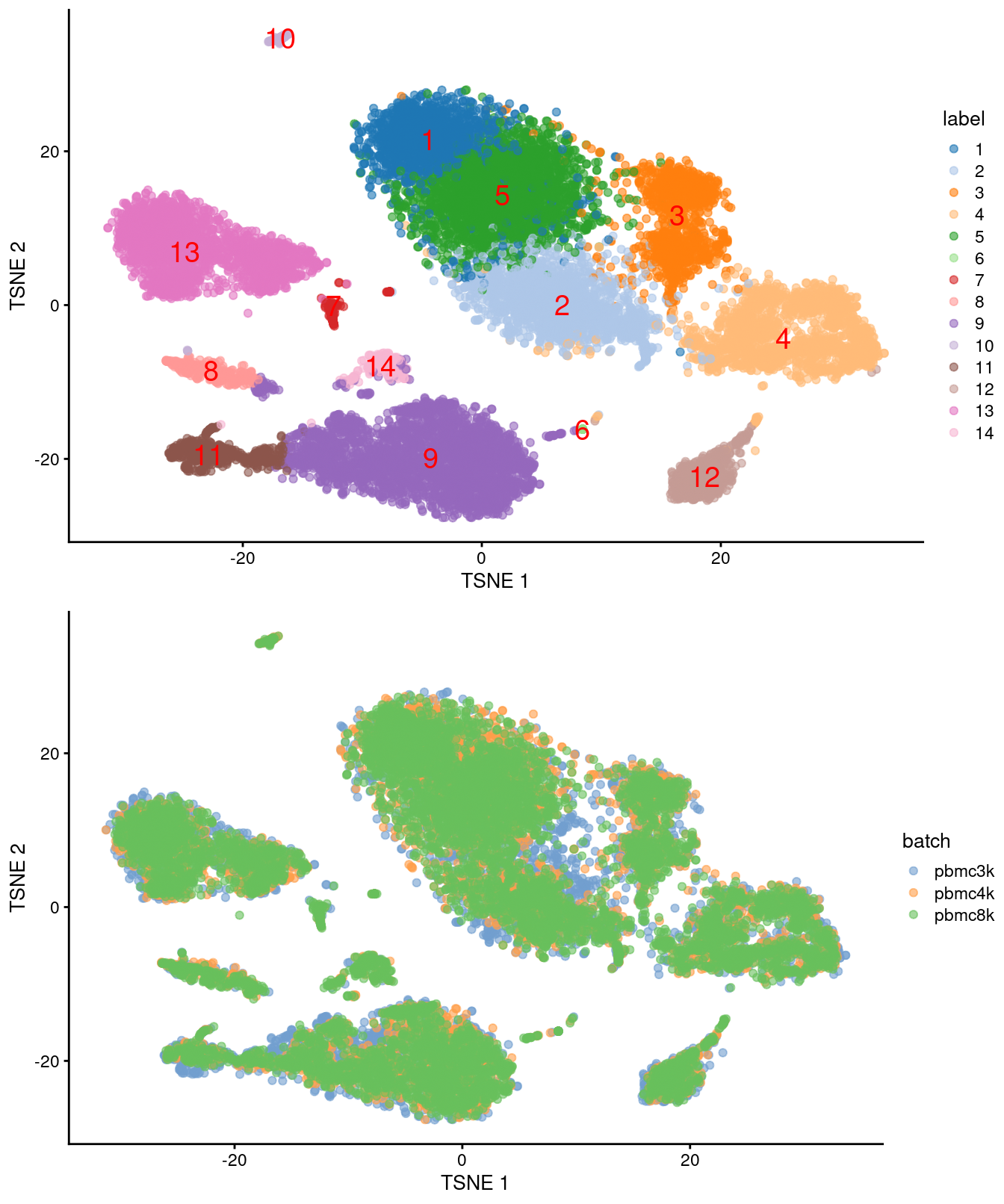
(\#fig:unref-filtered-pbmc-merged-tsne)Obligatory $t$-SNE plots for the merged PBMC datasets, where each point represents a cell and is colored by cluster (top) or batch (bottom).

## Session Info {-}
``` R version 4.1.0 beta (2021-05-03 r80259) Platform: x86_64-pc-linux-gnu (64-bit) Running under: Ubuntu 20.04.2 LTS Matrix products: default BLAS: /home/biocbuild/bbs-3.14-bioc/R/lib/libRblas.so LAPACK: /home/biocbuild/bbs-3.14-bioc/R/lib/libRlapack.so locale: [1] LC_CTYPE=en_US.UTF-8 LC_NUMERIC=C [3] LC_TIME=en_GB LC_COLLATE=C [5] LC_MONETARY=en_US.UTF-8 LC_MESSAGES=en_US.UTF-8 [7] LC_PAPER=en_US.UTF-8 LC_NAME=C [9] LC_ADDRESS=C LC_TELEPHONE=C [11] LC_MEASUREMENT=en_US.UTF-8 LC_IDENTIFICATION=C attached base packages: [1] parallel stats4 stats graphics grDevices utils datasets [8] methods base other attached packages: [1] batchelor_1.9.0 BiocSingular_1.9.0 [3] scran_1.21.1 scater_1.21.0 [5] ggplot2_3.3.3 scuttle_1.3.0 [7] TENxPBMCData_1.11.0 HDF5Array_1.21.0 [9] rhdf5_2.37.0 DelayedArray_0.19.0 [11] Matrix_1.3-3 SingleCellExperiment_1.15.1 [13] SummarizedExperiment_1.23.0 Biobase_2.53.0 [15] GenomicRanges_1.45.0 GenomeInfoDb_1.29.0 [17] IRanges_2.27.0 S4Vectors_0.31.0 [19] BiocGenerics_0.39.0 MatrixGenerics_1.5.0 [21] matrixStats_0.58.0 BiocStyle_2.21.0 [23] rebook_1.3.0 loaded via a namespace (and not attached): [1] AnnotationHub_3.1.0 BiocFileCache_2.1.0 [3] igraph_1.2.6 BiocParallel_1.27.0 [5] digest_0.6.27 htmltools_0.5.1.1 [7] viridis_0.6.1 fansi_0.4.2 [9] magrittr_2.0.1 memoise_2.0.0 [11] ScaledMatrix_1.1.0 cluster_2.1.2 [13] limma_3.49.0 Biostrings_2.61.0 [15] colorspace_2.0-1 blob_1.2.1 [17] rappdirs_0.3.3 xfun_0.23 [19] dplyr_1.0.6 crayon_1.4.1 [21] RCurl_1.98-1.3 jsonlite_1.7.2 [23] graph_1.71.0 glue_1.4.2 [25] gtable_0.3.0 zlibbioc_1.39.0 [27] XVector_0.33.0 Rhdf5lib_1.15.0 [29] scales_1.1.1 DBI_1.1.1 [31] edgeR_3.35.0 Rcpp_1.0.6 [33] viridisLite_0.4.0 xtable_1.8-4 [35] dqrng_0.3.0 bit_4.0.4 [37] rsvd_1.0.5 ResidualMatrix_1.3.0 [39] metapod_1.1.0 httr_1.4.2 [41] FNN_1.1.3 dir.expiry_1.1.0 [43] ellipsis_0.3.2 pkgconfig_2.0.3 [45] XML_3.99-0.6 farver_2.1.0 [47] CodeDepends_0.6.5 sass_0.4.0 [49] uwot_0.1.10 dbplyr_2.1.1 [51] locfit_1.5-9.4 utf8_1.2.1 [53] tidyselect_1.1.1 labeling_0.4.2 [55] rlang_0.4.11 later_1.2.0 [57] AnnotationDbi_1.55.0 munsell_0.5.0 [59] BiocVersion_3.14.0 tools_4.1.0 [61] cachem_1.0.5 generics_0.1.0 [63] RSQLite_2.2.7 ExperimentHub_2.1.0 [65] evaluate_0.14 stringr_1.4.0 [67] fastmap_1.1.0 yaml_2.2.1 [69] knitr_1.33 bit64_4.0.5 [71] purrr_0.3.4 KEGGREST_1.33.0 [73] sparseMatrixStats_1.5.0 mime_0.10 [75] compiler_4.1.0 beeswarm_0.3.1 [77] filelock_1.0.2 curl_4.3.1 [79] png_0.1-7 interactiveDisplayBase_1.31.0 [81] tibble_3.1.2 statmod_1.4.36 [83] bslib_0.2.5.1 stringi_1.6.2 [85] highr_0.9 RSpectra_0.16-0 [87] lattice_0.20-44 bluster_1.3.0 [89] vctrs_0.3.8 pillar_1.6.1 [91] lifecycle_1.0.0 rhdf5filters_1.5.0 [93] BiocManager_1.30.15 jquerylib_0.1.4 [95] RcppAnnoy_0.0.18 BiocNeighbors_1.11.0 [97] cowplot_1.1.1 bitops_1.0-7 [99] irlba_2.3.3 httpuv_1.6.1 [101] R6_2.5.0 bookdown_0.22 [103] promises_1.2.0.1 gridExtra_2.3 [105] vipor_0.4.5 codetools_0.2-18 [107] assertthat_0.2.1 withr_2.4.2 [109] GenomeInfoDbData_1.2.6 grid_4.1.0 [111] beachmat_2.9.0 rmarkdown_2.8 [113] DelayedMatrixStats_1.15.0 Rtsne_0.15 [115] shiny_1.6.0 ggbeeswarm_0.6.0 ```